Geochronology
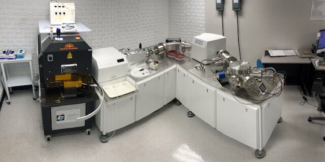
Arizona LaserChron Center Photon Machines Analyte-G2 ArF 193 nm excimer laser with a HelEx sample cell connected to a Nu plasma high-resolution (HR) multicollector mass spectrometer via aerosol rapid introduction system (ARIS). Photo: Martin Pepper.
Rapid U-Pb Zircon Geochronology by Laser Ablation Multicollector ICP-MS
at the arizona laserchron center

We are constantly striving to innovate at the Arizona LaserChron Center. This project focuses on increasing the rate of data acquisition of zircon U-Pb dates via multicollector LA-ICP-MS. The impetus for this project stems from the benefits of large-n detrital zircon geochronology.

Four methods for rapid acquisition of zircon U-Pb dates at rates of (a) 120 analyses/h, (b) 300 analyses/h, (c) 600 analyses/h, and (d) 1,200 analyses/h. All methods are time resolved analysis (TRA) at 0.2 s resolution where 1 index = 0.2 s. Data shown here are background subtracted. Time zero (t0) is the time laser firing begins and has a resolution of ± 0.2 s; background subtraction and on-peak measurements do not include indexes immediately before and after t0. Downhole correction is applied for the 120 analyses/h rate due to the long 15 s ablation time, all other acquisition methods use total counts (see Data Reduction section). Each plot shows real data from a test analytical session. Wash. = washout. Back. = background. Sundell et al. (2020), Geostandards and Geoanalytical Research.

Time resolved analysis (TRA) plotted as time series for the first 90 s of sample measurement from Session 1 on April 19, 2019. (a) 120 analyses/h (30s/analysis): background measurements are applied sample by sample. (b) 300 analyses/h (12s/analysis): background measurements are grouped for every 4 samples. (c) 600 analyses/h (6s/analysis): background measurements are grouped for every 10 samples. (d) 1,200 analyses/h (3s/analysis): background measurements are grouped for every 25 samples. Sundell et al. (2020), Geostandards and Geoanalytical Research.

Age offset plots. Circles = Session 1 (runs 1–4) on April 19, 2019. Squares = Session 2 (runs 5 – 8) April 20, 2019. (a) 120 analyses/h (30s/analyses) includes downhole correction, all other methods are calculated with total counts. (b) 300 analyses/h (12s/analysis). (c) 600 analyses/h (6s/analysis). (d) 1,200 analyses/h (3s/analysis). Offset is calculated as measured date – ID-TIMS date; left of 0% is young offset and right of 0% is old offset. Dates < 1,200 Ma are 206Pb/238U and ages > 1,200 Ma are 206Pb/207Pb. Random uncertainties are 1σ. Sundell et al. (2020), Geostandards and Geoanalytical Research.

Concordia diagrams. Purple ellipses are 1,200 analyses/h (3s/analysis). Green ellipses are 600 analyses/h (6s/analysis). Blue ellipses are 300 analyses/h (12s/analysis). Red ellipses are 120 analyses/h (30s/analysis). All uncertainty ellipses are 2σ. See Table 2 for reference material information. Note that the young reference materials (FCT and GHR1) are slightly positively discordant. This is because a compromise has to be made in the common Pb correction. Specifically, all panels in this figure share the same concordia line, and forcing these young zircons concordant by increasing the severity of the common Pb correction results in positively discordant older reference materials (e.g., Tan-Br-A and OG1). Sundell et al. (2020), Geostandards and Geoanalytical Research.

Results for detrital sample CP40 (Dickinson and Gehrels 2008). Age distributions for eight separate analytical sessions. The same number of zircons were analyzed at each rate (i.e., 120 unknowns were analyzed at 120 analyses/h; 300 unknowns were analyzed at 300 analyses/h). Y-axis probability corresponds only to probability density plots (PDP). Kernel density estimates (KDE) were constructed using a 15 Myr bandwidth. CC = Cross-correlation. L = Likeness. S = Similarity. All quantitative comparisons were calculated using DZstats (Saylor and Sundell 2016) version 2.3 for macOS. Sundell et al. (2020), Geostandards and Geoanalytical Research.

Three-dimensional multidimensional scaling (MDS) plot of results from then detrital application (see Section 5). Red circles = 120 analyses/h; blue circles = 300 analyses/h; green circles = 600 analyses/h; purple circles = 1,200 analyses/h; white circle = all accepted dates produced in this study. Black arrows correspond to the nearest neighbor. The comparison metric used is 1 – Cross correlation of Kernel density estimates (KDE) with a 15 Myr bandwidth to produce dissimilarity measure used to produce the MDS plot. Sundell et al. (2020), Geostandards and Geoanalytical Research.

Arizona LaserChron Center Nu plasma high-resolution (HR) multicollector mass spectrometer. Photo: Martin Pepper.